

In 2024, Nature Physics published a paper by Qian Xu, J. Pablo Bonilla Ataides and others titled Constant-overhead fault-tolerant quantum computation with reconfigurable atom arrays — a proposal to implement hypergraph product codes on neutral atom arrays.
The key insight, as the paper puts it, is that -
The product structure of one of the prototypical qLDPC codes, HGP codes, naturally matches the product structure of crossed AOD optical hardware, enabling its hardware-efficient implementation
I wrote some Python code to reproduce a few of the paper’s results, and this article explains it. The code of my work can be found at the GitHub repository.
The paper’s methods section provides the formula for computing the hypergraph product of two classical codes:
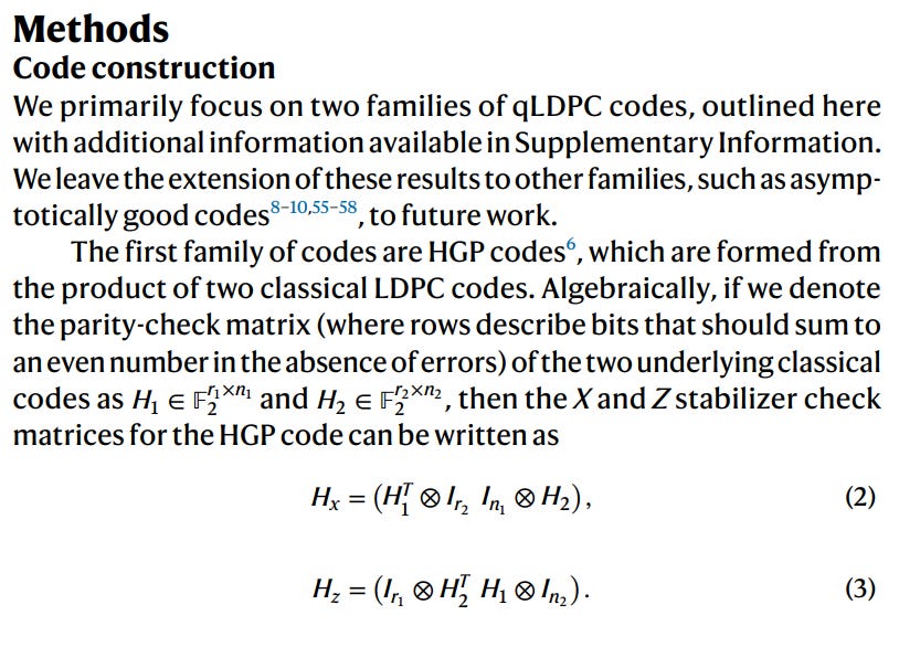
To implement this, I wrote the hypergraph function:
def hypergraph(H1, H2):
    """Hypergraph product of two classical codes. Returns (Hx, Hz)."""
    H1 = H1.copy().astype(np.uint8) % 2
    H2 = H2.copy().astype(np.uint8) % 2
    r1, n1 = H1.shape
    r2, n2 = H2.shape
    def I(k):
        return np.eye(k, dtype=np.uint8)
    Hx = np.hstack([np.kron(np.transpose(H1), I(r2)),
                    np.kron(I(n1), H2)])
    Hz = np.hstack([np.kron(I(r1), np.transpose(H2)),
                    np.kron(H1, I(n2))])
    return Hx, Hz
But which classical codes do we feed as inputs to this function? The paper then tells us exactly which classical codes we are HGP-ing together:
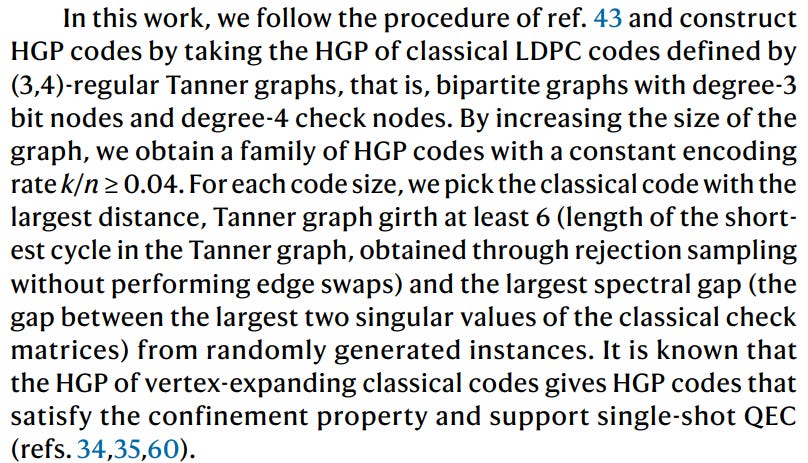
So we generate a random (3, 4)-regular Tanner graph and look at the corresponding parity check matrix. To do this, I defined the function regular_seed:
def regular_seed(n_bits, wc=3, wr=4, seed=0):
    """Random (wc, wr)-regular parity check matrix"""
    assert (n_bits * wc) % wr == 0
    r = n_bits * wc // wr
    bit_stubs   = np.repeat(np.arange(n_bits), wc)   # [0,0,0,1,1,1,2,2,2,...]
    check_stubs = np.repeat(np.arange(r), wr)        # [0,0,0,0,1,1,1,1,2,2,2,2,...]
    rng = np.random.default_rng(seed)
    while True:
        rng.shuffle(bit_stubs)
        H = np.zeros((r, n_bits), dtype=np.uint8)
        for i in range(n_bits * wc):
            H[check_stubs[i], bit_stubs[i]] += 1
        if np.all(H <= 1):
            break
    assert np.all(np.sum(H, axis=0) == wc) # assert the column sums are all wc
    assert np.all(np.sum(H, axis=1) == wr) # assert the row sums are all wr
    return H
But the condition “(3, 4)-regular Tanner graph” specifies an entire ensemble of classical codes. The regular_seed function just produced a random matrix from the ensemble. What if we want to produce a particular matrix from the ensemble that also satisfies some good properties? Indeed, the paper suggests the following criteria:
Filter the ensemble of (3, 4)-regular Tanner graphs to only consider Tanner graphs with girth ≥ 6. (This property is useful in decoding error syndromes.)
Within the set of (3, 4)-regular Tanner graphs with girth ≥ 6, prioritize those with the largest distance.
Within the set of (3, 4)-regular Tanner graphs with girth ≥ 6 and maximum distance, prioritize those with the largest spectral gap.
The standard way to do this — the way I tried doing it at first — is to first define the following functions:
def best_seed(n_bits, trials=100):
    """Sample many seeds, keep the one with the largest exact distance."""
    best_H, best_d = None, -1
    for s in range(trials):
        H = regular_seed(n_bits, wc=3, wr=4, seed=s)
        d = exact_distance(H)
        if d > best_d:
            best_H, best_d = H, d
    return best_H, best_d

def has_four_cycle(H):
    """True iff two checks share two or more bits. Equivalent to girth < 6."""
    G = H.astype(np.int64) @ H.astype(np.int64).T
    np.fill_diagonal(G, 0)
    return bool((G >= 2).any())

def spectral_gap(H):
    """sigma_1 - sigma_2 of H"""
    s = np.linalg.svd(H.astype(float), compute_uv=False)
    return float(s[0] - s[1])
And then run a flow chart algorithm like this:

Unfortunately, this doesn’t work so well in practice, because the proportion of (3, 4)-regular Tanner graphs that have girth ≥ 6 is quite small, so one would have to wait a long time to generate enough graphs. In particular, this is related to the Poisson distribution, which is beyond the scope of this article. But the key result is that
One could, of course, just brute force search for a long time. But I used a different approach instead — constructing graphs with girth ≥ 6 from the get-go, using the following progressive edge growth function:
def regular_seed_girth6(n_bits, rng, wc=3, wr=4, attempts=200):
    """A random (wc,wr)-regular seed whose Tanner graph has girth >= 6.

    girth >= 6 iff no two bits share more than one check.  We enforce that
    edge by edge while building: walk the bits in random order and,
    for each of its wc edges, connect it to
    the least-loaded check that would not close a 4-cycle."""

    r = n_bits * wc // wr
    for _ in range(attempts):
        H       = np.zeros((r, n_bits), dtype=np.uint8)
        rowd    = [0] * r                          # bits placed in each check
        co      = [set() for _ in range(n_bits)]   # bits sharing a check with b
        members = [[] for _ in range(r)]
        order   = list(range(n_bits))
        rng.shuffle(order)
        ok = True

        for b in order:
            for _edge in range(wc):
                cand = [c for c in range(r)
                        if rowd[c] < wr                     # check not yet full
                        and H[c, b] == 0                    # no repeated edge
                        and not (co[b] & set(members[c]))]  # no 4-cycle
                if not cand:
                    ok = False
                    break
                lo = min(rowd[c] for c in cand)             # least-loaded check
                cand = [c for c in cand if rowd[c] == lo]   # random tie-break
                c = cand[rng.randrange(len(cand))]

                H[c, b] = 1
                for x in members[c]:
                    co[x].add(b)
                    co[b].add(x)
                members[c].append(b)
                rowd[c] += 1
            if not ok:
                break

        if ok and all(d == wr for d in rowd):
            return H
    raise RuntimeError(f"no girth-6 seed at n_bits={n_bits} in {attempts} attempts")
By construction, this function always gives us (3, 4)-regular Tanner graphs with girth ≥ 6. Excellent!
Now, I run a search function that uses regular_seed_girth6 to generate many samples of such graphs, and then optimize for distance and spectral gap to give the final seed that we desired.
def search(n_bits, draws=1000, seed=0):
    """Returns (best_H, record).
    record holds (d, gap, k1, rank) for every accepted draw"""

    rng = random.Random(seed)
    record, best_H, best_key = [], None, None

    for _ in range(draws):
        H = regular_seed_girth6(n_bits, rng)   # girth >= 6 by construction
        assert not has_four_cycle(H)           # cheap independent confirmation

        k1  = nullspace(H).shape[0]
        d   = exact_distance(H)
        gap = spectral_gap(H)
        record.append({"d": d, "gap": gap, "k1": k1, "rank": n_bits - k1})

        key = (d, gap)                         # distance first, gap as tie-break
        if best_key is None or key > best_key:
            best_key, best_H = key, H

    return best_H, record
Finally, we have good classical seeds that we can take the HGP of. Here, I take the best classical matrix returned by the search function and take the HGP with itself.
Now, the only question remains, what size n of bits should we take? To answer this, I look at the codes that the paper uses. Figure 3 a of the paper gives the codes:
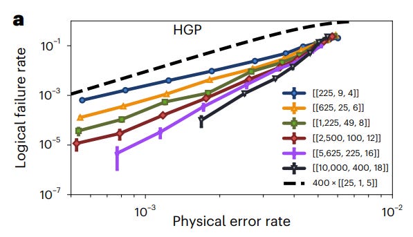
Reading from the figure, we see that the codes used by the paper are [[225, 9, 4]], [[625, 25, 6]], [[1225, 49, 8]], [[2500, 100, 12]], [[5625, 225, 16]], and [[10000, 400, 18]].
Now, we must reverse-engineer the classical seed that would give us an HGP code with parameters [[225, 9, 4]], and we will later repeat this for the other codes too.
Let Hseed be a classical (3, 4)-regular parity check matrix that we will use as a ‘seed’ in the hypergraph product. Suppose Hseed acts on nseed bits, and assume H has full rank. We would like to know, how many checks rseed does Hseed have? How many physical qubits nqubits does the HGP have? How many logical qubits kqubits does the HGP have? What is the rate kqubits / nqubits of the HGP code?
We can count the checks rseed two different ways using the (3, 4)-regular property: 3n or 4r. Setting these equal, we get
The number of message bits of the classical code Hseed is then
Recalling that the hypergraph product places qubits on check × check and bit × bit positions, we get that the physical qubit count of the HGP is
and the logical qubit count of the HGP is
So rate of the HGP code is
Observe that the rate is independent of n — this is exactly the “constant overhead” in the paper’s title.
But the paper says that the rate of the HGP code is lower-bounded by 0.04, why is that?
If Hseed has full rank, then the number of checks (i.e., number of rows) rseed = rank(Hseed), and the rate of the HGP code is exactly 0.04. But in the general case,
Now, back to the task of reverse-engineering, we want nqubits = 225 and kqubits = 9, so
Repeating similarly for the other codes, we find that
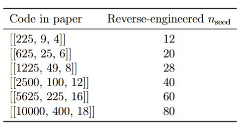
Once I got these nseed values, I ran my search function to reproduce the codes used by the paper. Here are my results:
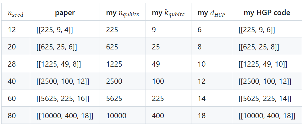
I am not sure why I got a higher distance than the paper in the cases of nseed being 12, 20, and 28. In all likelihood, there is some error in my code that I am trying to find out. In the case nseed = 60, I got a lower distance than the paper, presumably because I searched only 1000 samples.
Next, I also cross-checked Table 1 of the paper, which tells us their calculation of the overhead savings in using HGP or LP codes over the surface code.
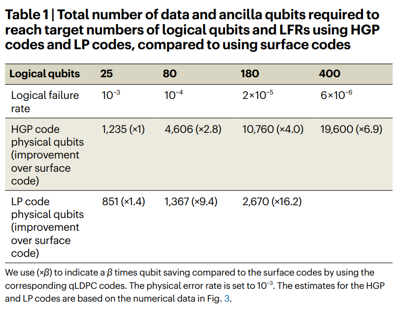
We will focus on the row about HGP codes. From the above results, we already know that 25 logical qubits ←→ nseed = 20 and 400 logical qubits ←→ nseed = 80. So let us try to understand where the corresponding physical qubit counts for those HGP codes (1,235 and 19,600 respectively) come from.
We already know that a (3, 4)-regular seed on nseed bits gives an HGP code with 25/16 n2seed data qubits. Syndrome extraction needs one ancilla atom per stabilizer generator, so how many ancilla qubits do we have?
Well, recalling that HGP places stabilizers on check × bit and bit × check positions, the number of stabilizer generators (i.e., the number of ancilla qubits) is
So the total number of physical qubits is data qubits + ancilla qubits, which gives us
And indeed, plugging in nseed = 20 gives total qubits = 1,225 (a disagreement with the 1,235 figure in the table) and plugging in nseed = 80 gives total qubits = 19,600.
To conclude this article, here are some questions and observations I had while working on this project -
It is not clear to me from reading the paper whether they took HGP of a good seed code with itself, or HGP of two different good seed codes.
It is not clear to me from reading the paper whether they first generated entire sets of (3, 4)-regular Tanner graphs and then rejected those with girth ≤ 4, or they too used a progressive edge growth algorithm to deliberately construct only those (3, 4)-regular Tanner graphs that already have girth ≥ 6.
In Table 1, I had a disagreement with the paper for total qubits for an HGP code at 25 logical qubits (paper says 1,235 v/s my result of 1,225). Also, 80 and 180 are not k2 for any integer k, so perhaps they interpolated the fit to a continuous code size? Or maybe they used HGP of two different seed codes (perhaps with something like k1 = 8 and k2 = 10)
While distance and spectral gap had a maximisation constraint, girth only had a threshold. We were not trying to maximise girth, instead we were allowing everything above threshold girth ( ≥ 6). To understand this better, I will look into how exactly decoders rely on the no-4-cycle property.
In the flow chart for seed generation, we did not optimise for low-rank (say, non-full rank) even though low rank improves the code rate. What if we include a rank-minimisation criteria in the seed generation algorithm?
Why exactly do we maximise spectral gap?
It would be interesting to see what fraction of criteria-satisfying seeds of a given size come out full rank.